Quantum Pseudo-Telepathy

1. Overview

In this article, we explore the concept of quantum pseudo-telepathy through the magic square game, a non-local game that demonstrates how quantum strategies using entanglement can outperform classical ones. Quantum pseudo-telepathy is often regarded as a thought experiment to highlight the non-local characteristics of quantum mechanics, but it is also a real-world phenomenon that can be experimentally verified. As such, it serves as a striking example of the experimental confirmation of Bell inequality violations. We examine how classical strategies are limited to a success probability of \(8/9\), while a carefully designed quantum strategy leveraging entanglement can achieve a 100% success rate. We also explore why the order of measurements in the quantum strategy does not affect the outcome, which is central to achieving perfect success in the game.

2. The Magic Square Game

The Magic Square Game is a cooperative game between two players, Alice and Bob, played on a \(3 \times 3\) grid. The referee assigns Alice to choose a row and Bob to choose a column, and both players must fill the grid with \(\pm 1\) values. Their goal is to ensure that:

• Alice’s row has an even number of \(-1\), ensuring the product of entries is \(+1\).
• Bob’s column has an odd number of \(-1\), ensuring the product of entries is \(-1\).

Crucially, Alice and Bob are not allowed to communicate once the game begins, and they must ensure that the value at the intersection of Alice’s row and Bob’s column is consistent for both players. While they can agree on a strategy beforehand, this restriction adds significant difficulty to the game.

3. Classical Limitations

In a classical strategy, Alice and Bob may try to prearrange a table with \(\pm 1\) values, but it is impossible for any classical configuration to consistently satisfy both players’ constraints. This arises because the parity conditions on the rows and columns inherently conflict: the rows must have an even number of \(-1\), while the columns must have an odd number of \(-1\). When attempting to construct a \(3 \times 3\) table that satisfies these conditions, a contradiction is bound to emerge. Specifically, at most eight slots can be made to fit the constraints, but the final slot will always conflict with either the row or column condition.

As a result, the best classical strategy can achieve a maximum success probability of \(8/9\). This occurs when Alice and Bob’s answers match in all but one cell of the grid. The inherent limitation of classical strategies demonstrates the gap between classical and quantum approaches, where quantum entanglement allows for perfect success in the Magic Square Game.

4. Quantum Advantage: 100% Success

In contrast to the classical strategy, a quantum strategy allows Alice and Bob to share a maximally entangled state and use quantum measurements to win the game with a 100% success rate. This is achieved through the use of carefully designed commuting observables, which allow Alice and Bob to align their measurements in a way that ensures the success conditions are met.

4.1 Initial Entangled State

The quantum strategy involves Alice and Bob sharing a maximally entangled state \(\ket{\Psi}\) composed of two Bell pairs, represented by:

\[\ket{\Psi} = \ket{\Phi^+}_{1,2} \otimes \ket{\Phi^+}_{3,4} = \frac{1}{2} \left( \ket{0000} + \ket{0011} + \ket{1100} + \ket{1111} \right)\]

where each Bell state is defined as:

\[\ket{\Phi^+}_{a,b} = \frac{1}{\sqrt{2}} \left( \ket{00}_{a,b} + \ket{11}_{a,b} \right)\]

In this setup, Alice holds qubits 1 and 3, while Bob holds qubits 2 and 4. Depending on the row (for Alice) or column (for Bob) they are assigned, they will measure specific observables that guarantee the game’s rules are satisfied.

4.2 Quantum Strategy for 100% Success

In the quantum strategy, Alice and Bob are able to achieve a 100% success rate by measuring specific observables that are carefully designed to satisfy the game’s conditions. The operators they measure are chosen from a predetermined set of commuting observables, as illustrated in the figure below.

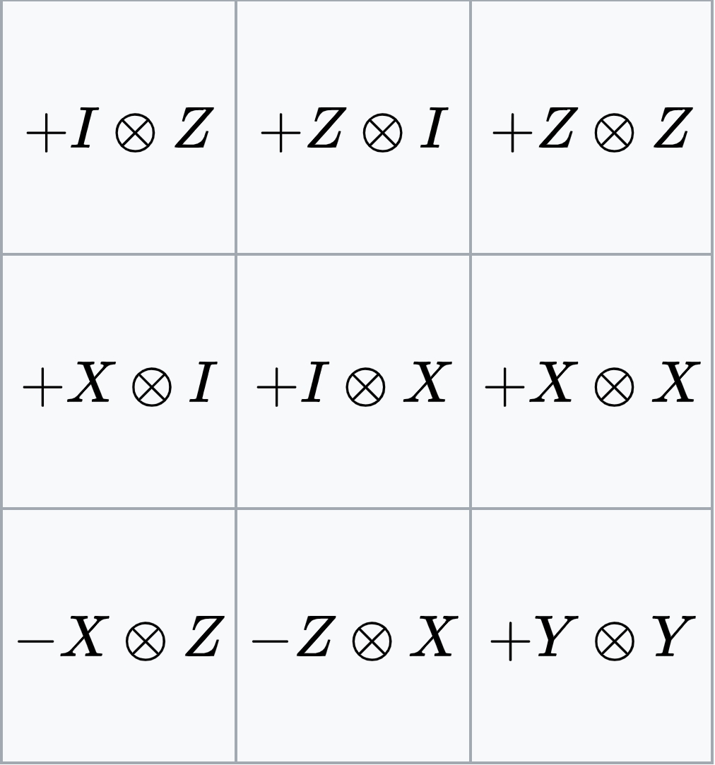Figure 1: The set of commuting observables used in the quantum strategy for the Magic Square Game. Each row corresponds to Alice’s measurements, while each column corresponds to Bob’s measurements.

In this strategy:

• Alice measures the observables corresponding to the rows of the matrix.
• Bob measures the observables corresponding to the columns of the matrix.

For example:

• In the first row, Alice’s measurements are \(X \otimes I\), \(X \otimes X\), and \(I \otimes X\), which commute with one another.
• In the first column, Bob’s measurements are \(X \otimes I\), \(-X \otimes Z\), and \(I \otimes Z\), which also commute.

The key feature of the quantum strategy is that these carefully chosen observables always satisfy the winning conditions of the Magic Square Game:

• Alice’s row measurements always yield a product of \(+1\), ensuring that she has an even number of \(-1\) in her row.
• Bob’s column measurements always yield a product of \(-1\), ensuring that he has an odd number of \(-1\) in his column.

By using the entangled state \(\ket{\Psi}\) and measuring these commuting observables, Alice and Bob can ensure that their values in the shared slot always match, and the game’s requirements are satisfied with 100% success. This quantum strategy highlights a significant advantage over classical approaches, which are limited to a success probability of \(8/9\).

In the following discussion, we will explain why performing measurements according to this grid of commuting observables (as in Figure 1) leads to guaranteed success. We will begin by introducing the concept of commuting observables and proceed to show how the calculated expectation values perfectly match the conditions of the game.

4.3 Commuting Observables and Game Design

The success of the quantum strategy is based on the fact that Alice’s and Bob’s observables for each row and column are commuting operators. The commuting property has two important implications:

• First, the operators within each player’s row (for Alice) or column (for Bob) commute, meaning that the order of measurements within each row or column does not affect the overall probability distribution of outcomes. Although the specific results of each measurement may differ (since each measurement collapses the state), the probability distribution remains the same. Alice can measure her observables in any order, and Bob can do the same, without influencing the overall distribution of their outcomes.
• Second, the operators corresponding to Alice’s rows and Bob’s columns also commute, ensuring that Alice’s measurements do not disturb Bob’s measurements, and vice versa. This allows them to measure their respective observables independently without affecting the overall game outcome.

Two operators commute if their commutator is zero:

\[[\hat{A}, \hat{B}] = \hat{A}\hat{B} - \hat{B}\hat{A} = 0\]

This property ensures that measurements can be performed independently of their order or timing, whether by Alice or Bob. For example, Alice’s first row consists of the following operators:

\[I \otimes Z, \quad Z \otimes I, \quad Z \otimes Z\]

These operators commute with each other, meaning that Alice can measure them in any order, and while the specific outcomes of each measurement may vary (due to state collapse), the overall probability distribution will remain the same. Similarly, Bob’s first column involves:

\[I \otimes Z, \quad X \otimes I, \quad -X \otimes Z\]

These operators also commute with one another, ensuring that Bob can perform his measurements in any order without affecting the overall probability distribution of his results.

The critical aspect of the quantum strategy is that the operators for Alice and Bob also commute across different qubits. This ensures that their measurements do not interfere with each other, preserving the quantum correlations necessary for the game’s success.

While many of the operators, especially in the first rows and columns, have an evident commutation structure, there is one particular set of operators—\(X \otimes X\), \(Y \otimes Y\), and \(Z \otimes Z\)—in a column that requires more careful analysis to see why they commute. These operators might not immediately appear to commute due to their structure, which motivates a deeper investigation.

4.4 Commutator Derivations for \(X \otimes X\), \(Y \otimes Y\), and \(Z \otimes Z\)

In the quantum strategy, Alice and Bob measure observables such as \(X \otimes X\), \(Y \otimes Y\), and \(Z \otimes Z\). These tensor products commute with each other, meaning they can be measured simultaneously without conflict. Let’s derive this in detail.

4.4.1 Commutator of \(X \otimes X\) and \(Y \otimes Y\):

\[[X \otimes X, Y \otimes Y] = (X \otimes X)(Y \otimes Y) - (Y \otimes Y)(X \otimes X)\]

First, calculate \((X \otimes X)(Y \otimes Y)\):

\[(X \otimes X)(Y \otimes Y) = (\sigma_x \otimes \sigma_x)(\sigma_y \otimes \sigma_y) = (\sigma_x \sigma_y) \otimes (\sigma_x \sigma_y) = (i \sigma_z) \otimes (i \sigma_z) = -(Z \otimes Z)\]

Next, calculate \((Y \otimes Y)(X \otimes X)\):

\[(Y \otimes Y)(X \otimes X) = (\sigma_y \otimes \sigma_y)(\sigma_x \otimes \sigma_x) = (\sigma_y \sigma_x) \otimes (\sigma_y \sigma_x) = (-i \sigma_z) \otimes (-i \sigma_z) = -(Z \otimes Z)\]

Thus, the commutator is:

\[[X \otimes X, Y \otimes Y] = -(Z \otimes Z) - (-(Z \otimes Z)) = 0\]

4.4.2 Commutator of \(Y \otimes Y\) and \(Z \otimes Z\):

Similarly:

\[(Y \otimes Y)(Z \otimes Z) = (\sigma_y \otimes \sigma_y)(\sigma_z \otimes \sigma_z) = (-i \sigma_x) \otimes (-i \sigma_x) = -(X \otimes X)\] \[(Z \otimes Z)(Y \otimes Y) = (\sigma_z \otimes \sigma_z)(\sigma_y \otimes \sigma_y) = (i \sigma_x) \otimes (i \sigma_x) = -(X \otimes X)\]

Thus:

\[[Y \otimes Y, Z \otimes Z] = -(X \otimes X) - (-(X \otimes X)) = 0\]

4.4.3 Commutator of \(Z \otimes Z\) and \(X \otimes X\):

Finally:

\[(Z \otimes Z)(X \otimes X) = (\sigma_z \otimes \sigma_z)(\sigma_x \otimes \sigma_x) = (-i \sigma_y) \otimes (-i \sigma_y) = -(Y \otimes Y)\] \[(X \otimes X)(Z \otimes Z) = (\sigma_x \otimes \sigma_x)(\sigma_z \otimes \sigma_z) = (i \sigma_y) \otimes (i \sigma_y) = -(Y \otimes Y)\]

Thus:

\[[Z \otimes Z, X \otimes X] = -(Y \otimes Y) - (-(Y \otimes Y)) = 0\]

4.5 Commutativity only in Tensor Products of Pauli Matrices

It’s important to note that while individual Pauli matrices \(X\), \(Y\), and \(Z\) do not commute with each other, their tensor products, such as \(X \otimes X\), \(Y \otimes Y\), and \(Z \otimes Z\), do commute. For example:

\[[X, Y] = 2iZ \neq 0, \quad [Y, Z] = 2iX \neq 0, \quad [Z, X] = 2iY \neq 0\]

But:

\[[X \otimes X, Y \otimes Y] = [Y \otimes Y, Z \otimes Z] = [Z \otimes Z, X \otimes X] = 0\]

4.6 Commuting Observables and Measurement Order

A key aspect of the quantum strategy in the magic square game is the use of commuting observables within the rows and columns, as well as across different qubits. This ensures that Alice and Bob can measure their respective observables independently, without affecting each other’s results.

We have shown that the operators within Alice’s rows and Bob’s columns commute, ensuring that the order of measurements does not affect the overall outcome distribution. Additionally, since Alice and Bob’s observables act on different qubits, they commute across qubits as well. Mathematically, this is expressed as:

\[[A_i \otimes I, I \otimes B_j] = 0\]

where \(A_i\) is an observable Alice measures on her qubits, and \(B_j\) is an observable Bob measures on his qubits. The fact that these operators commute means that Alice and Bob can perform their measurements independently of each other, without affecting the outcome.

Given that both the observables within rows and columns, and the observables across Alice’s and Bob’s qubits, commute, it follows that each player can measure their assigned row or column in any order. This allows the entire game to be played with Alice and Bob performing their measurements at any time, in any order, without requiring any communication once the game has started. The independence and commutativity of the observables guarantee that all the necessary correlations are preserved, and the game’s rules are satisfied.

This commuting structure forms the foundation for why Alice and Bob can achieve a 100% success rate in the quantum strategy. The fact that every observable can be measured independently and in any order paves the way for the next step: calculating the expectation values of these measurements to show that Alice’s row measurements yield a product of \(+1\), and Bob’s column measurements yield a product of \(-1\), as required to win the game. Furthermore, these calculations will demonstrate that the values at the shared slot always match, ensuring the consistency needed for a perfect strategy.

4.7 Calculating Expectation Values

4.7.1 Row and Column Expectation Values

Now that we have established that the observables commute, we can calculate the expectation values of the measurements. For the game to be won, Alice’s row measurements must always yield a product of \(+1\) and Bob’s column measurements must yield a product of \(-1\).

Consider Alice’s first row, based on the observables in Figure 1. The product of the observables is:

\[(I \otimes Z)(Z \otimes I)(Z \otimes Z) = I \otimes I\]

We can compute the expectation value of the identity operator:

\[\braket{\Psi | I \otimes I | \Psi} = 1\]

Since the eigenvalues of Pauli matrices are \(\pm 1\), an expectation value of \(1\) for the product of the observables indicates that there is an even number of \(-1\) in the row. This confirms that Alice’s row satisfies the required condition. Similarly, we can verify that the other rows also yield the same result.

Likewise, for Bob’s first column:

\[(I \otimes Z)(X \otimes I)(-X \otimes Z) = -I \otimes I\]

The expectation value of this operator is:

\[\braket{\Psi | -I \otimes I | \Psi} = -1\]

This guarantees that Bob’s column always has an odd number of \(-1\). As with Alice, we can easily verify that other columns satisfy this result as well.

4.7.2 Why the Common Slot Matches for Both Players

Let’s now explain why Alice’s and Bob’s shared slot must always match. When Alice and Bob measure their respective observables on the same slot, the commuting nature of the observables ensures that they do not interfere with each other’s results. For instance, in the third row and second column, Alice and Bob measure the following observables:

\[O_A = -Z_1 \otimes X_3, \quad O_B = -Z_2 \otimes X_4\]

Given our previous discussion on commuting observables, we know that the order of the measurements does not affect the outcome distribution, since all the relevant operators commute. This allows us to calculate the expectation value using the initial state \(\ket{\Psi}\), rather than any post-measured state, as we can treat the shared slot as if it were measured first, without impacting the expectation value.

We now calculate the expectation value of the product of these two operators, \(O_A O_B\), acting on the initial state \(\ket{\Psi}\). Applying the product of these operators to the state:

\[(Z_1 \otimes Z_2 \otimes X_3 \otimes X_4) \ket{\Psi} = \ket{0011} + \ket{0000} + \ket{1111} + \ket{1100} = \ket{\Psi}\]

The expectation value of this product is:

\[\braket{\Psi | O_A O_B | \Psi} = \braket{\Psi | \Psi} = 1\]

This shows that the measurement outcomes of Alice and Bob are perfectly correlated at the shared slot, ensuring that their values always match. Similarly, we can easily verify that other shared slots satisfy this result as well. The game design, utilizing commuting observables, guarantees that the correlation is preserved and that the players win with a probability of 100%.

5. Conclusion

The Magic Square Game exemplifies the power of quantum mechanics, where quantum entanglement and non-locality enable Alice and Bob to succeed with certainty. By leveraging commuting observables and a shared entangled state, they achieve perfect coordination, something unattainable with classical strategies due to inherent conflicts in row and column parity.

This quantum advantage highlights the deep non-local correlations that exist in quantum systems. The game is a vivid example of how quantum mechanics can surpass classical limitations, offering practical insights into quantum pseudo-telepathy and the violation of Bell inequalities. Such non-locality is not only a theoretical curiosity but also a foundation for real-world applications, such as device-independent quantum key distribution (DIQKD). In DIQKD, similar non-local correlations can be used to establish secure communication protocols, even when the underlying devices are untrusted.

Ultimately, the Magic Square Game serves as a compelling demonstration of how quantum entanglement and commuting measurements can outperform classical approaches and opens the door to future applications in quantum cryptography and secure communications.